library(tidyverse)
#> ── Attaching core tidyverse packages ──────────────────────── tidyverse 2.0.0 ──
#> ✔ dplyr 1.2.1 ✔ readr 2.2.0
#> ✔ forcats 1.0.1 ✔ stringr 1.6.0
#> ✔ ggplot2 4.0.3 ✔ tibble 3.3.1
#> ✔ lubridate 1.9.5 ✔ tidyr 1.3.2
#> ✔ purrr 1.2.2
#> ── Conflicts ────────────────────────────────────────── tidyverse_conflicts() ──
#> ✖ dplyr::filter() masks stats::filter()
#> ✖ dplyr::lag() masks stats::lag()
#> ℹ Use the conflicted package (<http://conflicted.r-lib.org/>) to force all conflicts to become errorsCase Study: Glycoproteomics
An end-to-end glycoproteomics analysis with Glycoverse.
This vignette walks you through a complete glycoproteomics analysis using glycoverse. We’ll explore the full spectrum of glycoproteomics data analysis, from data loading and preprocessing to statistical analysis and visualization. We’ll also dive into advanced glycan structure analysis, including motif quantification and derived trait analysis. Ready to dive in? Let’s go!
Heads up: glycoverse is built on tidy principles throughout. If you’re new to tidyverse data analysis, we highly recommend checking out Hadley Wickham’s excellent R for Data Science. Trust us, it’s worth the investment!
Quick readiness check:
- What’s a
tibble? - How do you filter rows in a
tibble? - What’s the modern alternative to
forloops? - What’s the
|>operator? - What makes data “tidy”?
TL;DR
In case you’re in a hurry…
# Load the packages
library(tidyverse)
library(glycoverse)
library(SummarizedExperiment)

# Preprocess the data
clean_exp <- auto_clean(real_experiment)

# Perform PCA
pca_res <- gly_pca(clean_exp)
autoplot(pca_res)

# Perform differential expression analysis
limma_res <- gly_limma(clean_exp)
get_tidy_result(limma_res)

# Perform motif analysis
motifs <- c(
  lewis_by = "dHex(??-?)Hex(??-?)[dHex(??-?)]HexNAc(??-",
  lewis_ax = "Hex(??-?)[dHex(??-?)]HexNAc(??-",
  sia_lewis_ax = "NeuAc(??-?)Hex(??-?)[dHex(??-?)]HexNAc(??-"
)
motif_exp <- quantify_motifs(clean_exp, motifs)
motif_anova_res <- gly_anova(motif_exp)
get_tidy_result(motif_anova_res, "main_test")

# Perform derived trait analysis
trait_exp <- derive_traits(clean_exp)
trait_anova_res <- gly_anova(trait_exp)
get_tidy_result(trait_anova_res, "main_test")
Loading the Packages
We first load the tidyverse package, as usual.
Just like tidyverse, glycoverse is a meta-package that loads a collection of specialized packages all at once.
library(glycoverse)
#> ── Attaching core glycoverse packages ────────────────────── glycoverse 0.3.1 ──
#> ✔ glyclean 0.15.1     ✔ glyparse 0.7.1
#> ✔ glydet   0.12.1     ✔ glyread  0.12.0
#> ✔ glydraw  0.6.3      ✔ glyrepr  0.13.0
#> ✔ glyexp   0.16.0     ✔ glystats 0.11.1
#> ✔ glymotif 0.17.1     ✔ glyvis   0.7.1
#> ── Conflicts ───────────────────────────────────────── glycoverse_conflicts() ──
#> ✖ glyclean::aggregate()  masks stats::aggregate()
#> ✖ dplyr::filter()        masks stats::filter()
#> ✖ lubridate::intersect() masks dplyr::intersect(), base::intersect()
#> ✖ dplyr::lag()           masks stats::lag()
#> ✖ lubridate::setdiff()   masks dplyr::setdiff(), base::setdiff()
#> ✖ dplyr::setequal()      masks base::setequal()
#> ✖ lubridate::union()     masks dplyr::union(), base::union()
#> ℹ Use the conflicted package (<http://conflicted.r-lib.org/>) to force all conflicts to become errors
The Glycoverse data containers extend SummarizedExperiment, so we load it to use its standard accessors.
library(SummarizedExperiment)
#> Loading required package: MatrixGenerics
#> Loading required package: matrixStats
#>
#> Attaching package: 'matrixStats'
#> The following object is masked from 'package:dplyr':
#>
#>     count
#>
#> Attaching package: 'MatrixGenerics'
#> The following objects are masked from 'package:matrixStats':
#>
#>     colAlls, colAnyNAs, colAnys, colAvgsPerRowSet, colCollapse,
#>     colCounts, colCummaxs, colCummins, colCumprods, colCumsums,
#>     colDiffs, colIQRDiffs, colIQRs, colLogSumExps, colMadDiffs,
#>     colMads, colMaxs, colMeans2, colMedians, colMins, colOrderStats,
#>     colProds, colQuantiles, colRanges, colRanks, colSdDiffs, colSds,
#>     colSums2, colTabulates, colVarDiffs, colVars, colWeightedMads,
#>     colWeightedMeans, colWeightedMedians, colWeightedSds,
#>     colWeightedVars, rowAlls, rowAnyNAs, rowAnys, rowAvgsPerColSet,
#>     rowCollapse, rowCounts, rowCummaxs, rowCummins, rowCumprods,
#>     rowCumsums, rowDiffs, rowIQRDiffs, rowIQRs, rowLogSumExps,
#>     rowMadDiffs, rowMads, rowMaxs, rowMeans2, rowMedians, rowMins,
#>     rowOrderStats, rowProds, rowQuantiles, rowRanges, rowRanks,
#>     rowSdDiffs, rowSds, rowSums2, rowTabulates, rowVarDiffs, rowVars,
#>     rowWeightedMads, rowWeightedMeans, rowWeightedMedians,
#>     rowWeightedSds, rowWeightedVars
#> Loading required package: GenomicRanges
#> Loading required package: stats4
#> Loading required package: BiocGenerics
#> Loading required package: generics
#>
#> Attaching package: 'generics'
#> The following object is masked from 'package:lubridate':
#>
#>     as.difftime
#> The following object is masked from 'package:dplyr':
#>
#>     explain
#> The following objects are masked from 'package:base':
#>
#>     as.difftime, as.factor, as.ordered, intersect, is.element, setdiff,
#>     setequal, union
#>
#> Attaching package: 'BiocGenerics'
#> The following object is masked from 'package:dplyr':
#>
#>     combine
#> The following objects are masked from 'package:stats':
#>
#>     IQR, mad, sd, var, xtabs
#> The following objects are masked from 'package:base':
#>
#>     anyDuplicated, aperm, append, as.data.frame, basename, cbind,
#>     colnames, dirname, do.call, duplicated, eval, evalq, Filter, Find,
#>     get, grep, grepl, is.unsorted, lapply, Map, mapply, match, mget,
#>     order, paste, pmax, pmax.int, pmin, pmin.int, Position, rank,
#>     rbind, Reduce, rownames, sapply, saveRDS, table, tapply, unique,
#>     unsplit, which.max, which.min
#> Loading required package: S4Vectors
#>
#> Attaching package: 'S4Vectors'
#> The following objects are masked from 'package:lubridate':
#>
#>     second, second<-
#> The following objects are masked from 'package:dplyr':
#>
#>     first, rename
#> The following object is masked from 'package:tidyr':
#>
#>     expand
#> The following object is masked from 'package:utils':
#>
#>     findMatches
#> The following objects are masked from 'package:base':
#>
#>     expand.grid, I, unname
#> Loading required package: IRanges
#>
#> Attaching package: 'IRanges'
#> The following object is masked from 'package:lubridate':
#>
#>     %within%
#> The following objects are masked from 'package:dplyr':
#>
#>     collapse, desc, slice
#> The following object is masked from 'package:purrr':
#>
#>     reduce
#> Loading required package: Seqinfo
#> Loading required package: Biobase
#> Welcome to Bioconductor
#>
#>     Vignettes contain introductory material; view with
#>     'browseVignettes()'. To cite Bioconductor, see
#>     'citation("Biobase")', and for packages 'citation("pkgname")'.
#>
#> Attaching package: 'Biobase'
#> The following object is masked from 'package:MatrixGenerics':
#>
#>     rowMedians
#> The following objects are masked from 'package:matrixStats':
#>
#>     anyMissing, rowMedians
#> The following object is masked from 'package:glyexp':
#>
#>     samples
Reading the Data
Data import is typically your first step in any analysis. For this tutorial, we’ll use the real_experiment dataset that comes with glyexp. This is a real-world N-glycoproteomics dataset from 12 patients across four liver conditions: healthy controls (H), hepatitis (M), cirrhosis (Y), and hepatocellular carcinoma (C), with 3 samples per condition.
real_experiment
#>
#> ── GlycoproteomicSE ────────────────────────────────────────────────────────────
#> ℹ Abundance assay: 12 samples, 4262 variables
#> ℹ Glycan type: N
#> ℹ Row data fields: peptide <chr>, peptide_site <int>, protein <chr>, protein_site <int>, gene <chr>, glycan_composition <comp>, glycan_structure <struct>
#> ℹ Column data fields: group <fct>
#> ℹ Metadata fields: exp_type <chr>, glycan_type <chr>, quant_method <chr>
For your own projects, the glyread package can import data from virtually any mainstream glycoproteomics software—pGlyco3, MSFragger-Glyco, Byonic, you name it. Each software has its own dedicated import function. For instance, data from pGlyco3 with pGlycoQuant quantification can be loaded using read_pglyco3_pglycoquant(). Check out Get Started with glyread for the full rundown.
The real_experiment object is a GlycoproteomicSE object. Glycoverse import functions return this specialized SummarizedExperiment for glycoproteomics data. It manages three key components:
- Abundance assay: quantitative data with samples as columns and variables as rows
- Column data: sample metadata (group, batch, demographics, etc.)
- Row data: feature metadata (proteins, peptides, glycan compositions, etc.)
You can access these components with assay(), colData(), and rowData().
assay(real_experiment)[1:5, 1:5]
#>                                              C1         C2           C3
#> P08185-176-Hex(5)HexNAc(4)NeuAc(2)           NA         NA     10655.62
#> P04196-344-Hex(5)HexNAc(4)NeuAc(1)-1  414080036  609889761  78954431.49
#> P04196-344-Hex(5)HexNAc(4)            581723113  604842244 167889901.32
#> P04196-344-Hex(5)HexNAc(4)NeuAc(1)-2 3299649335 2856490652 957651065.86
#> P10909-291-Hex(6)HexNAc(5)-1           30427048   34294394   6390129.81
#>                                                H1         H2
#> P08185-176-Hex(5)HexNAc(4)NeuAc(2)   3.105412e+04         NA
#> P04196-344-Hex(5)HexNAc(4)NeuAc(1)-1           NA   11724908
#> P04196-344-Hex(5)HexNAc(4)           6.977076e+08  703566323
#> P04196-344-Hex(5)HexNAc(4)NeuAc(1)-2 2.600523e+09 3229968280
#> P10909-291-Hex(6)HexNAc(5)-1 5.159133e+07 37479075as_tibble(colData(real_experiment))
#> # A tibble: 12 × 1
#> group
#> <fct>
#> 1 C
#> 2 C
#> 3 C
#> 4 H
#> 5 H
#> 6 H
#> 7 M
#> 8 M
#> 9 M
#> 10 Y
#> 11 Y
#> 12 Yas_tibble(rowData(real_experiment))
#> # A tibble: 4,262 × 7
#> peptide peptide_site protein protein_site gene glycan_composition
#> <chr> <int> <chr> <int> <chr> <comp>
#> 1 NKTQGK 1 P08185 176 SERPINA6 Hex(5)HexNAc(4)Neu…
#> 2 HSHNNNSSDLHPHK 5 P04196 344 HRG Hex(5)HexNAc(4)Neu…
#> 3 HSHNNNSSDLHPHK 5 P04196 344 HRG Hex(5)HexNAc(4)
#> 4 HSHNNNSSDLHPHK 5 P04196 344 HRG Hex(5)HexNAc(4)Neu…
#> 5 HNSTGCLR 2 P10909 291 CLU Hex(6)HexNAc(5)
#> 6 HSHNNNSSDLHPHK 5 P04196 344 HRG Hex(5)HexNAc(4)Neu…
#> 7 HSHNNNSSDLHPHK 6 P04196 345 HRG Hex(5)HexNAc(4)
#> 8 HSHNNNSSDLHPHK 5 P04196 344 HRG Hex(5)HexNAc(4)dHe…
#> 9 HSHNNNSSDLHPHK 5 P04196 344 HRG Hex(4)HexNAc(3)
#> 10 HSHNNNSSDLHPHK 5 P04196 344 HRG Hex(4)HexNAc(4)Neu…
#> # ℹ 4,252 more rows
#> # ℹ 1 more variable: glycan_structure <struct>For a deeper dive into Glycoverse data containers, check out Get Started with glyexp.
Data Preprocessing
Raw quantification data needs preprocessing before analysis—that’s just a fact of life in omics. Typical steps include normalization, missing value imputation, and batch effect correction. Rather than making you implement these tedious steps manually, glyclean provides a comprehensive preprocessing pipeline. Just call auto_clean() on your GlycoproteomicSE object and you’re good to go.
clean_exp <- auto_clean(real_experiment)
#>
#> ── Removing variables with too many missing values ──
#>
#> ℹ Applying preset "discovery"...
#> ℹ Total removed: 24 (0.56%) variables.
#> ✔ Variable removal completed.
#>
#> ── Normalizing data ──
#>
#> ℹ Normalization method: `normalize_median()`
#> ℹ Reason: default for "glycoproteomics".
#> ✔ Normalization completed.
#>
#> ── Imputing missing values ──
#>
#> ℹ Imputation method: `impute_min_prob()`
#> ℹ Reason: default for "glycoproteomics" with n_samples < 30.
#> ✔ Imputation completed.
#>
#> ── Aggregating data ──
#>
#> ℹ Aggregating to "gfs" level
#> ✔ Aggregation completed.
#>
#> ── Normalizing data again ──
#>
#> ℹ Normalization method: `normalize_median()`
#> ℹ Reason: default for "glycoproteomics".
#> ✔ Normalization completed.
#>
#> ── Correcting batch effects ──
#>
#> ℹ Batch column batch not found in sample_info. Skipping batch correction.
#> ✔ Batch correction completed.
Your data is now analysis-ready!
Want to customize the preprocessing steps? See Get Started with glyclean for the full toolkit.
Statistical Analysis and Visualization
Time for the fun part—statistical analysis and visualization! We’ll use glystats for the number crunching and glyvis to make sense of the results visually.
Let’s kick off with PCA to get a bird’s-eye view of our data structure.
plot_pca(clean_exp) # from `glyvis`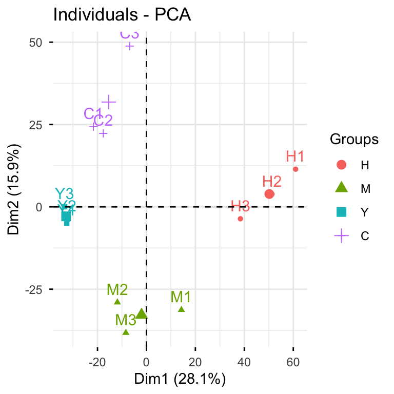
glyvis isn’t designed for publication-ready figures, but it’s perfect for quick exploratory visualization. Behind the scenes, plot_pca() calls gly_pca() from glystats and renders the results.
You can also break this down into separate steps:
pca_res <- gly_pca(clean_exp)  # from `glystats`
autoplot(pca_res)  # from `glyvis`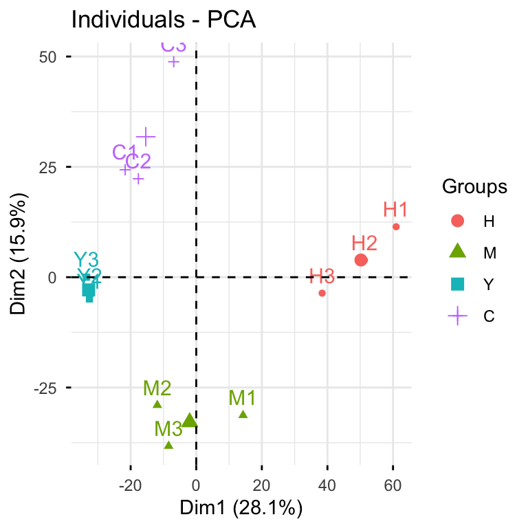
# you can also use `plot_pca(pca_res)`We actually recommend the two-step approach, since it gives you more flexibility with the results. You can create custom ggplot2 visualizations for publications or extract the underlying data when reviewers ask for it.
glystats covers virtually all standard omics analyses. All functions follow the same naming pattern: gly_xxx()—think gly_anova(), gly_ttest(), gly_roc(), gly_cox(), gly_wgcna(), and so on. They take a GlycomicSE, GlycoproteomicSE, or compatible SummarizedExperiment as their first argument.
The return format is consistent across all functions—a list with two components:
tidy_result: cleaned-up tibbles in tidy format. We’ve done the heavy lifting of organizing messy statistical output for you.raw_result: the original statistical objects. These are available when you need to dig deeper or perform advanced analyses.
glystats provides two helper functions to get the tidy result tibble and the raw result list from a glystats result object: get_tidy_result() and get_raw_result(). Let’s now see what the samples tibble looks like:
get_tidy_result(pca_res, "samples")  # many tibbles, so we specify one of them
#> # A tibble: 144 × 4
#>    sample group    PC  value
#>    <chr>  <fct> <dbl>  <dbl>
#>  1 C1     C         1 -21.7
#>  2 C1     C         2  24.3
#>  3 C1     C         3   1.46
#>  4 C1     C         4   1.10
#>  5 C1     C         5  11.4
#>  6 C1     C         6 -24.8
#>  7 C1     C         7  -5.62
#>  8 C1     C         8   2.45
#>  9 C1     C         9  28.3
#> 10 C1     C        10  -9.73
#> # ℹ 134 more rows
Notice the “group” column? That’s glystats being helpful— it automatically pulls relevant metadata from your GlycoproteomicSE object and includes it in the results wherever it makes sense.
Back to that autoplot() magic we saw earlier. It automatically recognizes different glystats result types and plots accordingly— no manual specification needed. The plots won’t win any beauty contests, but they’ll get your data insights across fast.
The PCA clearly shows that our samples cluster nicely by condition—always a good sign! Now let’s dive into differential expression analysis using the tried-and-true limma package.
limma_res <- gly_limma(clean_exp, contrasts = "H_vs_C")  # from `glystats`
#> ℹ Number of groups: 4
#> ℹ Groups: "H", "M", "Y", and "C"
#> ℹ Pairwise comparisons will be performed, with levels coming first as reference groups.
get_tidy_result(limma_res)  # only one tibble here
#> # A tibble: 3,979 × 14
#>    variable       protein glycan_composition glycan_structure protein_site gene
#>    <chr>          <chr>   <comp>             <struct>                <int> <chr>
#>  1 P08185-176-He… P08185  Hex(5)HexNAc(4)Ne… NeuAc(??-?)Hex(…          176 SERP…
#>  2 P04196-344-He… P04196  Hex(5)HexNAc(4)Ne… NeuAc(??-?)Hex(…          344 HRG
#>  3 P04196-344-He… P04196  Hex(5)HexNAc(4)    Hex(??-?)HexNAc…          344 HRG
#>  4 P04196-344-He… P04196  Hex(5)HexNAc(4)Ne… NeuAc(??-?)Hex(…          344 HRG
#>  5 P10909-291-He… P10909  Hex(6)HexNAc(5)    Hex(??-?)HexNAc…          291 CLU
#>  6 P04196-344-He… P04196  Hex(5)HexNAc(4)Ne… NeuAc(??-?)Hex(…          344 HRG
#>  7 P04196-345-He… P04196  Hex(5)HexNAc(4)    Hex(??-?)HexNAc…          345 HRG
#>  8 P04196-344-He… P04196  Hex(5)HexNAc(4)dH… dHex(??-?)Hex(?…          344 HRG
#>  9 P04196-344-He… P04196  Hex(4)HexNAc(3)    Hex(??-?)HexNAc…          344 HRG
#> 10 P04196-344-He… P04196  Hex(4)HexNAc(4)Ne… NeuAc(??-?)Hex(…          344 HRG
#> # ℹ 3,969 more rows
#> # ℹ 8 more variables: log2fc <dbl>, AveExpr <dbl>, t <dbl>, p_val <dbl>,
#> #   p_adj <dbl>, b <dbl>, ref_group <chr>, test_group <chr>
Excellent! Now let’s identify significantly differentially expressed glycoforms between HCC and healthy samples, then see what biological pathways they’re involved in.
library(glyfun)

limma_res |>
  enrich_ora_go(dea_p_cutoff = 0.05, dea_log2fc_cutoff = c(-2, 2)) |>
  clusterProfiler::dotplot()
#>
#>
#> 'select()' returned 1:1 mapping between keys and columns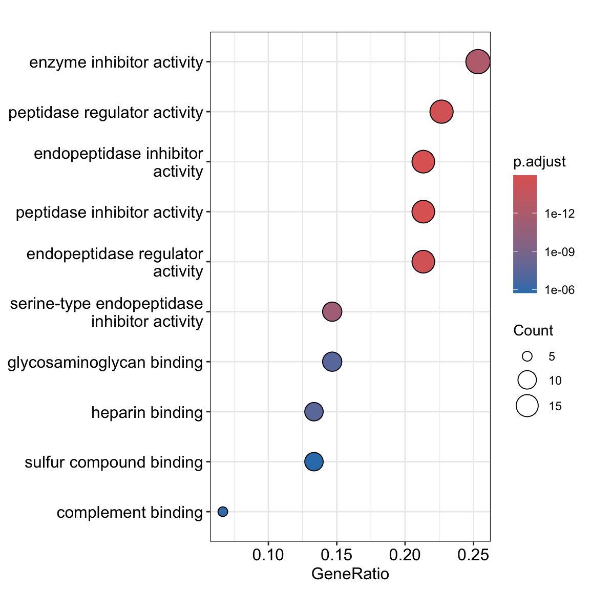
And that’s it—pathway enrichment in just a few lines! We used enrich_ora_go() from glyfun to perform GO over-representation analysis on the significant hits from our gly_limma() results. glyfun is not a core glycoverse package, so you need to load it separately.
For the full statistical arsenal, check out Get Started with glystats and Get Started with glyvis. To explore more functional enrichment options, see Get Started with glyfun.
Advanced Motif Analysis
Up to now, we’ve covered standard glycoproteomics workflows. While glycoverse certainly streamlines these analyses, it truly shines when it comes to advanced glycan structure analysis.
Before diving into motifs, let’s get acquainted with glyrepr::glycan_structure() vectors.
clean_exp |>
  rowData() |>
  as_tibble() |>
  pull(glycan_structure)
#> <glycan_structure[3979]>
#> [1] NeuAc(??-?)Hex(??-?)HexNAc(??-?)Hex(??-?)[NeuAc(??-?)Hex(??-?)HexNAc(??-?)Hex(??-?)]Hex(??-?)HexNAc(??-?)HexNAc(??-
#> [2] NeuAc(??-?)Hex(??-?)HexNAc(??-?)[HexNAc(??-?)]Hex(??-?)[Hex(??-?)Hex(??-?)]Hex(??-?)HexNAc(??-?)HexNAc(??-
#> [3] Hex(??-?)HexNAc(??-?)Hex(??-?)[Hex(??-?)HexNAc(??-?)Hex(??-?)]Hex(??-?)HexNAc(??-?)HexNAc(??-
#> [4] NeuAc(??-?)Hex(??-?)HexNAc(??-?)Hex(??-?)[Hex(??-?)HexNAc(??-?)Hex(??-?)]Hex(??-?)HexNAc(??-?)HexNAc(??-
#> [5] Hex(??-?)HexNAc(??-?)Hex(??-?)HexNAc(??-?)Hex(??-?)[Hex(??-?)HexNAc(??-?)Hex(??-?)]Hex(??-?)HexNAc(??-?)HexNAc(??-
#> [6] NeuAc(??-?)Hex(??-?)HexNAc(??-?)Hex(??-?)[NeuAc(??-?)Hex(??-?)HexNAc(??-?)Hex(??-?)]Hex(??-?)HexNAc(??-?)HexNAc(??-
#> [7] Hex(??-?)HexNAc(??-?)Hex(??-?)[Hex(??-?)HexNAc(??-?)Hex(??-?)]Hex(??-?)HexNAc(??-?)HexNAc(??-
#> [8] dHex(??-?)Hex(??-?)HexNAc(??-?)Hex(??-?)[dHex(??-?)Hex(??-?)HexNAc(??-?)Hex(??-?)]Hex(??-?)HexNAc(??-?)HexNAc(??-
#> [9] Hex(??-?)HexNAc(??-?)Hex(??-?)[Hex(??-?)]Hex(??-?)HexNAc(??-?)HexNAc(??-
#> [10] NeuAc(??-?)Hex(??-?)HexNAc(??-?)Hex(??-?)[HexNAc(??-?)Hex(??-?)]Hex(??-?)HexNAc(??-?)HexNAc(??-
#> ... (3969 more not shown)
#> # Unique structures: 967
Just like integer() and character(), glycan_structure() is a specialized vector type. Some software (like pGlyco3 and StrucGP) outputs structural information as text strings. When you import this data using glyread, the glyparse package automatically converts these strings into proper glycan_structure() vectors and stores them in the variable information tibble. Note that not all software provides structural data—some only give compositions.
Fortunately, our example dataset includes structural information, opening up a world of advanced analytical possibilities. Let’s explore motif analysis.
Quick note: The printed structures use IUPAC-condensed notation, which we’ll also use for defining motifs below. Don’t worry if it looks intimidating—we’ll include visual diagrams to help. That said, if you’re planning to do serious structural analysis, learning IUPAC-condensed notation is worth the investment. Check out this guide to get started—it’s easier than it looks!
Lewis antigen epitopes are common structural motifs found on N-glycans. Ignoring linkage specificity, we can define three main Lewis motif families:
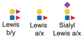
Here’s how we express these motifs in IUPAC-condensed notation:
motifs <- c(
  lewis_by = "dHex(??-?)Hex(??-?)[dHex(??-?)]HexNAc(??-",
  lewis_ax = "Hex(??-?)[dHex(??-?)]HexNAc(??-",
  sia_lewis_ax = "NeuAc(??-?)Hex(??-?)[dHex(??-?)]HexNAc(??-"
)
A couple of important points:
- We’re using generic monosaccharide names (“Hex” vs. “Glc”) to match typical glycoproteomics data resolution
- The “??-?” represents unknown linkages—a common limitation in mass spectrometry data
This level of structural ambiguity is typical in glycoproteomics. The key is matching your motif definitions to your data’s resolution.
Here’s our research question: How many glycosites show differential Lewis antigen expression across conditions? Without glycoverse, this would be a nightmare to tackle manually. Take a moment to imagine the pain of doing this by hand!
Now, the glycoverse solution:
motif_anova_res <- clean_exp |>
  quantify_motifs(motifs) |>  # quantify these motifs
  gly_anova()  # and perform ANOVA
#> ℹ Number of groups: 4
#> ℹ Groups: "H", "M", "Y", and "C"
#> ℹ Pairwise comparisons will be performed, with levels coming first as reference groups.

get_tidy_result(motif_anova_res, "main_test")
#> # A tibble: 828 × 15
#>    variable         protein protein_site trait gene  motif_structure term     df
#>    <chr>            <chr>          <int> <chr> <chr> <struct>        <chr> <dbl>
#>  1 A6NJW9-49-lewis… A6NJW9            49 lewi… CD8B2 dHex(??-?)Hex(… group     3
#>  2 A6NJW9-49-lewis… A6NJW9            49 lewi… CD8B2 Hex(??-?)[dHex… group     3
#>  3 A6NJW9-49-sia_l… A6NJW9            49 sia_… CD8B2 NeuAc(??-?)Hex… group     3
#>  4 O14786-150-lewi… O14786           150 lewi… NRP1  dHex(??-?)Hex(… group     3
#>  5 O14786-150-lewi… O14786           150 lewi… NRP1  Hex(??-?)[dHex… group     3
#>  6 O14786-150-sia_… O14786           150 sia_… NRP1  NeuAc(??-?)Hex… group     3
#>  7 O43866-226-lewi… O43866           226 lewi… CD5L  dHex(??-?)Hex(… group     3
#>  8 O43866-226-lewi… O43866           226 lewi… CD5L  Hex(??-?)[dHex… group     3
#>  9 O43866-226-sia_… O43866           226 sia_… CD5L  NeuAc(??-?)Hex… group     3
#> 10 O75437-244-lewi… O75437           244 lewi… ZNF2… dHex(??-?)Hex(… group     3
#> # ℹ 818 more rows
#> # ℹ 7 more variables: sumsq <dbl>, meansq <dbl>, statistic <dbl>, p_val <dbl>,
#> #   p_adj <dbl>, effect_size <dbl>, post_hoc <chr>
quantify_motifs() transforms your data into a new SummarizedExperiment. Instead of quantifying individual glycans per glycosite, you now have motif abundances per glycosite across samples. All glystats functions work seamlessly with this container—including gly_anova().
Now we can answer our question using standard tidyverse operations, since motif_anova_res$tidy_result$main_test is just a regular tibble:
motif_anova_res |>
  get_tidy_result("main_test") |>
  filter(p_adj < 0.05) |>
  group_by(trait) |>
  dplyr::count()
#> # A tibble: 3 × 2
#> # Groups:   trait [3]
#>   trait            n
#>   <chr>        <int>
#> 1 lewis_ax        18
#> 2 lewis_by         5
#> 3 sia_lewis_ax    19
Want the specific glycosites with significant Lewis a/x epitopes? Easy:
motif_anova_res |>
  get_tidy_result("main_test") |>
  filter(p_adj < 0.05, trait == "lewis_ax") |>
  select(protein, protein_site)
#> # A tibble: 18 × 2
#>    protein protein_site
#>    <chr>          <int>
#>  1 P00738           241
#>  2 P01011           271
#>  3 P01042           294
#>  4 P01877           205
#>  5 P01877            92
#>  6 P02675           394
#>  7 P02679            78
#>  8 P02749           162
#>  9 P02763            93
#> 10 P03952           494
#> 11 P04114          3411
#> 12 P05090            98
#> 13 P05156           177
#> 14 P05546            49
#> 15 P10909            86
#> 16 P20851            64
#> 17 P51884           127
#> 18 Q08380           125
glymotif has much more to offer beyond these examples. Dive deeper with Get Started with glymotif.
Derived Trait Analysis
Let’s wrap up with derived traits—a clever analytical approach developed by the N-glycomics community for glycome characterization. Classic examples include:
- High-mannose glycan proportion
- Core-fucosylation rate within complex glycans
- Average sialylation per galactose residue
glydet adapts this concept for glycoproteomics by treating each glycosite as its own mini-glycome. This enables site-specific trait calculation and much richer biological insights.
Using glydet couldn’t be simpler:
trait_exp <- derive_traits(clean_exp)  # from `glydet`
trait_exp
#> class: SummarizedExperiment
#> dim: 3864 12
#> metadata(3): exp_type glycan_type quant_method
#> assays(1): abundance
#> rownames(3864): A6NJW9-49-TM A6NJW9-49-TH ... Q9Y6W6-184-AG
#>   Q9Y6W6-184-TS
#> rowData names(5): protein protein_site trait gene explanation
#> colnames(12): C1 C2 ... Y2 Y3
#> colData names(1): group
That’s it! Just like quantify_motifs(), derive_traits() creates a new SummarizedExperiment, but now with trait values per glycosite per sample.
The variable information shows what we’re working with:
as_tibble(rowData(trait_exp))
#> # A tibble: 3,864 × 5
#>    protein protein_site trait gene  explanation
#>    <chr>          <int> <chr> <chr> <chr>
#>  1 A6NJW9            49 TM    CD8B2 Proportion of high-mannose glycans among al…
#>  2 A6NJW9            49 TH    CD8B2 Proportion of hybrid glycans among all glyc…
#>  3 A6NJW9            49 TC    CD8B2 Proportion of complex glycans among all gly…
#>  4 A6NJW9            49 MM    CD8B2 Abundance-weighted mean of mannose count wi…
#>  5 A6NJW9            49 CA2   CD8B2 Proportion of bi-antennary glycans within c…
#>  6 A6NJW9            49 CA3   CD8B2 Proportion of tri-antennary glycans within …
#>  7 A6NJW9            49 CA4   CD8B2 Proportion of tetra-antennary glycans withi…
#>  8 A6NJW9            49 TF    CD8B2 Proportion of fucosylated glycans among all…
#>  9 A6NJW9            49 TFc   CD8B2 Proportion of core-fucosylated glycans amon…
#> 10 A6NJW9            49 TFa   CD8B2 Proportion of arm-fucosylated glycans among…
#> # ℹ 3,854 more rows
The “trait” column lists all the derived traits we can analyze.
glydet comes with a comprehensive set of built-in traits:
TM: Proportion of high-mannose glycansTH: Proportion of hybrid glycansTC: Proportion of complex glycansMM: Average number of mannoses within high-mannose glycansCA2: Proportion of bi-antennary glycans within complex glycansCA3: Proportion of tri-antennary glycans within complex glycansCA4: Proportion of tetra-antennary glycans within complex glycansTF: Proportion of fucosylated glycansTFc: Proportion of core-fucosylated glycansTFa: Proportion of arm-fucosylated glycansTB: Proportion of glycans with bisecting GlcNAcSG: Average degree of sialylation per galactoseGA: Average degree of galactosylation per antennaTS: Proportion of sialylated glycans
These represent the most widely used traits in glycomics literature.
Let’s identify glycosites with significantly different core-fucosylation levels (TFc) across conditions:
trait_exp |>
  filter_row(trait == "TFc") |>  # from `glyexp`
  gly_anova() |>
  get_tidy_result("main_test") |>
  filter(p_adj < 0.05)
#> ℹ Number of groups: 4
#> ℹ Groups: "H", "M", "Y", and "C"
#> ℹ Pairwise comparisons will be performed, with levels coming first as reference groups.
#> # A tibble: 10 × 15
#>    variable     protein protein_site trait gene  explanation term     df   sumsq
#>    <chr>        <chr>          <int> <chr> <chr> <chr>       <chr> <dbl>   <dbl>
#>  1 P00748-249-… P00748           249 TFc   F12   Proportion… group     3 4.30e+0
#>  2 P01591-71-T… P01591            71 TFc   JCHA… Proportion… group     3 1.09e+0
#>  3 P02765-176-… P02765           176 TFc   AHSG  Proportion… group     3 1.65e+0
#>  4 P02790-240-… P02790           240 TFc   HPX   Proportion… group     3 4.25e-1
#>  5 P04004-86-T… P04004            86 TFc   VTN   Proportion… group     3 7.02e-1
#>  6 P05090-98-T… P05090            98 TFc   APOD  Proportion… group     3 8.62e-2
#>  7 P06681-621-… P06681           621 TFc   C2    Proportion… group     3 1.19e+2
#>  8 P0C0L4-1328… P0C0L4          1328 TFc   C4A   Proportion… group     3 5.21e+1
#>  9 P19652-103-… P19652           103 TFc   ORM2  Proportion… group     3 1.66e+1
#> 10 P20851-64-T… P20851            64 TFc   C4BPB Proportion… group     3 7.42e+1
#> # ℹ 6 more variables: meansq <dbl>, statistic <dbl>, p_val <dbl>, p_adj <dbl>,
#> #   effect_size <dbl>, post_hoc <chr>
Once again, it’s just that straightforward.
This just scratches the surface of glydet’s capabilities. The real power lies in defining custom traits tailored to your research questions. Explore the possibilities in Get Started with glydet.
What’s Next?
This vignette has given you a taste of glycoverse in action through a real-world glycoproteomics workflow. But we’ve barely scratched the surface! Now that you’ve got the basics down, you’re ready to unlock the full potential of each package.
Here’s your roadmap to mastering each component:
- glyexp — Master experiment objects and data manipulation
- glyread — Import and organize glycoproteomics data
- glyclean — Build custom preprocessing pipelines
- glystats — Explore the full statistical toolkit
- glyvis — Create stunning visualizations
- glymotif — Define and analyze custom motifs
- glydet — Create powerful derived traits
- glyenzy — Explore enzyme-substrate relationships (we didn’t cover this one, but it’s fascinating!)
- glyrepr — Master glycan structure representation
- glyparse — Parse and convert structural formats
- glydraw — Draw glycan structures
- glydb — Access glycan databases
- glyanno — Annotate glycan structures
- glyfun — Perform functional enrichment analysis
- glysmith — Master the full analytical pipeline
Happy glycan hunting! 🧬