Glycan Graphs: The Network Behind Glycan Structures

This vignette is for users who want to understand how glyrepr stores glycan structures internally. Some familiarity with graph theory and the igraph package will help. If those concepts are new to you, the igraph documentation is a useful companion reference.

Glycans as Graphs

Glycans are naturally represented as directed graphs. In glyrepr, an ordinary glycan structure is stored as an outward-directed tree, where each vertex represents a monosaccharide and each edge represents a glycosidic linkage. A structure with floating parts is stored as an annotated forest: one main tree plus one disconnected tree for each floating part.

Behind the scenes, each glycan_structure() object is backed by an igraph object. Most workflows can stay at the glycan_structure() level, but the graph representation is useful when you need custom structure analysis.

library(glyrepr)

What Is Stored in Memory?

A glycan can carry many kinds of information: linear oriented C-atoms, basetype, substituents, configuration, anomeric center, ring size, linkage positions, and more.

Some packages, such as Python’s glypy, store a very detailed glycan model. That comprehensive strategy is useful for specialized tasks such as MS/MS spectra simulation, but it can be overkill for everyday omics research.

glyrepr takes a more compact approach: if a feature can be derived from an IUPAC-condensed text representation, glyrepr stores it. Details such as configuration and ring size are not stored directly, because they are often predictable for common carbohydrates and are not needed for many glycomics workflows.

For a closer look at IUPAC-condensed notation, see the IUPAC-condensed vignette.

Extracting the Graph

You cannot pass a glycan_structure() object directly to most igraph functions. First, extract the underlying graph with get_structure_graphs():

glycan <- n_glycan_core()
graph <- get_structure_graphs(glycan)
graph
#> IGRAPH bc84ac4 DN-- 5 4 -- 
#> + attr: anomer (g/c), alditol (g/l), name (v/c), mono (v/c), sub (v/c),
#> | linkage (e/c)
#> + edges from bc84ac4 (vertex names):
#> [1] 3->1 3->2 4->3 5->4

The printed graph contains several pieces of information.

First line: Directed Named (“DN”) graph with 5 vertices (sugar units) and 4 edges (bonds).

Graph-level attributes:

anomer: the anomeric configuration of the reducing end.
alditol: whether the reducing-end residue is an alditol.
floating_parts, when present: virtual attachment metadata for disconnected floating components.
floating_substituents, when present: unresolved substituent tokens and their candidate parent residues.

Vertex attributes:

name: a unique ID for each monosaccharide.
mono: the monosaccharide type, such as “Hex” or “HexNAc”.
sub: chemical decorations attached to the monosaccharide.

Edge attributes:

linkage: how the monosaccharides are connected, including bond positions and configurations.

Connection pattern: “1->2” means vertex 1 connects to vertex 2. glyrepr treats bonds as arrows pointing from the core toward the branches. The direction is a modeling choice that makes traversal and structure operations easier.

You can also plot the graph with igraph:

plot(graph)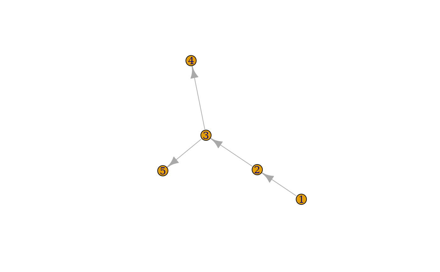

Graph Components

Vertices

Each vertex represents a monosaccharide with three key properties:

Names: These are auto-generated identifiers, usually simple integers, but they could be anything as long as they’re unique:

igraph::V(graph)$name
#> [1] "1" "2" "3" "4" "5"

Monosaccharides: These are IUPAC-condensed names like “Hex”, “HexNAc”, “Glc”, “GlcNAc”.

igraph::V(graph)$mono
#> [1] "Man"    "Man"    "Man"    "GlcNAc" "GlcNAc"

For the full list of available monosaccharides, check SNFG notation or run available_monosaccharides().

Substituents: Chemical decorations like “Me” (methyl), “Ac” (acetyl), “S” (sulfate), etc. Position matters. “3Me” = methyl at position 3, “?S” = sulfate at unknown position:

igraph::V(graph)$sub
#> [1] "" "" "" "" ""

Multiple decorations are comma-separated and sorted by position:

glycan2 <- as_glycan_structure("Glc3Me6S(a1-")
graph2 <- get_structure_graphs(glycan2)
igraph::V(graph2)$sub
#> [1] "3Me,6S"

Edges

Edges represent glycosidic bonds with a simple but powerful format:

<target anomeric config><target position> - <source position>

Here is an example where “Gal” has an “a” anomeric configuration, linking from position 3 of “GalNAc” to position 1 of “Gal”:

glycan3 <- as_glycan_structure("Gal(a1-3)GalNAc(b1-")
graph3 <- get_structure_graphs(glycan3)
igraph::E(graph3)$linkage
#> [1] "a1-3"

glyrepr stores anomer information in edges rather than vertices. This follows the way linkages are written in IUPAC-condensed notation, for example “Neu5Ac with an a2-3 linkage”.

Graph-Level Attributes

Anomer: The anomeric configuration of the reducing end.

graph$anomer
#> [1] "b1"

Alditol: Whether the reducing-end residue has been reduced. The attribute is always explicit on canonical graphs; legacy inputs without it are treated as FALSE. In IUPAC-condensed strings, -ol follows the reducing-end residue.

alditol <- as_glycan_structure("Gal(b1-4)GlcNAc-ol(a1-")
alditol_graph <- get_structure_graphs(alditol)
alditol_graph$alditol
#> [1] TRUE
get_alditol(alditol)
#> [1] TRUE

Floating Parts

A floating structure remains one igraph, but it is weakly disconnected. The floating-component vertices come first in complete IUPAC-condensed order, followed by the main-tree vertices in their canonical order.

floating <- as_glycan_structure(
  "{Neu5Ac(a2-3)|2,3}Gal(b1-3)[Gal(b1-4)]GlcNAc(a1-"
)
floating_graph <- get_structure_graphs(floating)

igraph::components(floating_graph, mode = "weak")$no
#> [1] 2
igraph::graph_attr(floating_graph, "floating_parts")
#> [[1]]
#> [[1]]$root
#> [1] 1
#> 
#> [[1]]$nodes
#> [1] 1
#> 
#> [[1]]$linkage
#> [1] "a2-3"
#> 
#> [[1]]$parents
#> [1] 2 3
structure_floating_parts(floating)
#> # A tibble: 1 × 6
#>   glycan_id part_id root_node nodes     linkage parents  
#>       <int>   <int>     <int> <list>    <chr>   <list>   
#> 1         1       1         1 <int [1]> a2-3    <int [2]>

Each floating_parts entry has four fields:

root: the vertex index at the root of the floating component.
nodes: every vertex index in the floating component.
linkage: the virtual linkage from that root to its unresolved parent.
parents: candidate vertex indices outside the component. integer() means all feasible nodes outside that component, including nodes in other floating parts. In a canonical structure, an explicit vector has at least two entries; a singleton is normalized to an ordinary edge.

These IDs follow complete IUPAC-condensed residue order: floating blocks are counted from left to right before the main glycan, and substituent blocks add no vertices. Component assignments must be acyclic and ultimately connect to the main tree.

The virtual attachment is not stored in igraph::E(floating_graph), because its endpoint is unresolved. Use structure_floating_parts() when a tabular representation must round-trip this metadata.

Floating Substituents

Floating substituents use the same candidate-parent convention without adding dummy vertices. Each floating_substituents entry contains substituent, such as "6S" or "?S", and parents. Empty parents means every feasible residue node in the complete structure, including floating-part nodes; otherwise the values are global graph vertex indices.

floating_sub <- as_glycan_structure(
  "{6S|1,2}Gal(a1-3)Glc(a1-3)Man(a1-"
)
floating_sub_graph <- get_structure_graphs(floating_sub)
igraph::graph_attr(floating_sub_graph, "floating_substituents")
#> [[1]]
#> [[1]]$substituent
#> [1] "6S"
#> 
#> [[1]]$parents
#> [1] 1 2
structure_floating_substituents(floating_sub)
#> # A tibble: 1 × 4
#>   glycan_id substituent_id substituent parents  
#>       <int>          <int> <chr>       <list>   
#> 1         1              1 6S          <int [2]>

Working with the Graph

Using `igraph`

Once you understand the graph structure, you can use igraph functions for custom structure analysis. Remember that tree-specific functions need special handling for a structure with floating parts: get_structure_graphs() and smap() pass the complete annotated forest, not only the main tree.

Example 1: Count branched structures (sugars with multiple children):

sum(igraph::degree(graph, mode = "out") > 1)
#> [1] 1

Example 2: Explore the structure with breadth-first search:

bfs_result <- igraph::bfs(graph, root = 1, mode = "out")
bfs_result$order
#> + 5/5 vertices, named, from bc84ac4:
#> [1] 1 2 3 4 5

Using `smap` Functions

Working with multiple glycans? You could use purrr:

library(purrr)

glycans <- c(n_glycan_core(), o_glycan_core_1(), o_glycan_core_2())
graphs <- get_structure_graphs(glycans)  # Extract graphs first
map_int(graphs, ~ igraph::vcount(.x))    # Then analyze
#> [1] 5 2 3

For glycan structure vectors, glyrepr’s smap functions are usually a better fit:

smap_int(glycans, ~ igraph::vcount(.x))  # Direct analysis, no intermediate step.
#> [1] 5 2 3

The main advantage of smap functions is how they handle duplicates. Real datasets often contain many repeated structures, and smap optimizes by processing unique structures once, then efficiently expanding results back to the original dimensions.

The smap vignette covers this workflow in more detail.

Motif Analysis with `glymotif`

One important application is identifying biologically meaningful motifs, or functional substructures. The glymotif package, built on this graph foundation, specializes in exactly this task.

See the glymotif introduction for examples.

Summary

In this vignette, you saw:

how glycan structures map to directed graphs.
what information is stored and what is deliberately omitted.
how to extract and inspect the underlying graphs.
how igraph, smap, and glymotif can build on this representation.

The graph representation might seem complex at first, but it’s this solid foundation that enables all the sophisticated glycan analysis capabilities in the glycoverse. Most users will not need to manipulate the graph directly, but understanding the model makes it easier to extend glyrepr when custom analysis is needed.